- Tham gia
- 4/11/07
- Bài viết
- 14,656
- Được thích
- 37,341
- Donate (Momo)

- Giới tính
- Nam
- Nghề nghiệp
- Consultant
PART 2:CALCULATING WITH EXCEL
CREATE EASIER-TO-UNDERSTAND FORMULAS WITH NAMED RANGES
TẠO NHỮNG CÔNG THỨC DỄ HIỂU VỚI TÊN RANGE
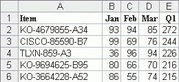
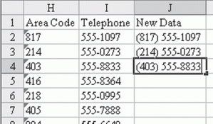
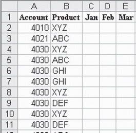
Problem: As shown in Fig. 206, your worksheet contains several different for­mulas. It would be easier to understand the results if each component of every formula were named for what it repre­sented and not just for the cell it came from.
Vấn đề: Như hình 206, bảng tính của bạn bao gồm rất nhiều công thức. Sẽ dễ hiểu hơn cái kết quả của các công thức này nếu mỗi thành phần của công thức được đặt tên theo nội dung của nó.
Fig. 206
Strategy: Use named ranges to make formulas easier to understand.
Give cell B3 a name of Revenue. Select cell B3. In the Name box (the area to the left of the formula bar), type Revenue and press Enter, as shown in Fig. 207.
Giải pháp: Sử dụng các range được đặt tên làm cho công thức dễ hiểu hơn.
Đặt tên cho cell B3 là Revenue (DoanhThu): Chọn cel B3, Trong hộp tên, (là ô ngoài cùng phía trái của thanh công thức), gõ Revenue và Enter như hình 207
Fig. 207
Give cell B4 a name of COGS.
Select cell B4. Click in the name box, type COGS and hit Enter.
Đặt tên cho cell B4 là COGS (Giá vốn COGS = Cost Of Goods Saled): Chọn cell B4, trong hộp Name Box, gõ COGS, và Enter.
Clear the formula in B6. Re-enter the formula and use the mouse to select the cells. Type an Equal sign. Using the mouse, touch B3. Type a Minus sign. Using the mouse, touch B4. This will enter the formula as =Revenue–COGS, as shown in Fig. 208. This is easier to understand than a typical formula.
Xoá công thức trong cell B6, Nhập lại công thức: Gõ dấu bằng (=), Dùng chuột chọn ô B3, gõ dấu trừ, dùng chuột chọn ô B4. Công thức sẽ là: = Renenue – COGS như hình 208. Sẽ dễ hiểu hơn là công thức thông thường.
Fig. 208
Gotcha: You need a lot of foresight to use this technique. In order to have this work automatically, you are supposed to be smart enough to create the range names before you enter the formula. However, most people get the formula first and then decide to make the worksheet eas­ier to understand.
1) If you want to assign names after the formulas are created, use In­sert – Name – Apply to apply names to existing formulas, as shown in Fig. 209.
Ghi chú: Bạn phải có tầm nhìn rộng khi sử dụng kỹ thuật này. Nhằm mục đích cho các tên này hoạt động tự động, bạn phải đủ ý thức để tạo những tên trước khi viết công thức. Dù vậy, người ta thường tạo công thức trước, sau đó mới tính đến chuyện làm cho bảng tính trở nên dễ hiểu.
Nếu bạn muốn áp các tên mới đặt vào các cộng thức có sẵn, hãy dùng Menu Insert – Name – Apply để áp các tên vào công thức có sẵn như hình 209
Fig. 209
2) As shown in Fig. 210, select all of the names that you want to apply.
Xem hình 210, chọn mọi cái tên mà bạn muốn áp vào công thức.
Fig. 210
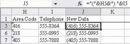
Result: A formula like =B6–B11 will be updated to =GrossProfit–Expenses, as shown in Fig. 211.
Kết quả: 1 công thức như là =B6-B11 sẽ được cập nhật thành =GrossProfit-Ex_Pense như hình 211 (Lãi gộp – Chi tiêu khác)
Fig. 211
Summary: To create plain language formulas, first assign a range name to each cell in your formula. Use the mouse when entering the formula. To assign range names to a formula after the fact, use Insert – Name – Apply.
Tóm tắt: Muốn tạo các công thức biết nói, trước tiên đặt tên cho các cell trong các công thức. Dùng chuột chọn cell khi tạo công thức. Muốn cập nhật các tên mới đặt cho các công thức có sẵn, dùng Menu Insert – Name – Apply.
CREATE EASIER-TO-UNDERSTAND FORMULAS WITH NAMED RANGES
TẠO NHỮNG CÔNG THỨC DỄ HIỂU VỚI TÊN RANGE
Problem: As shown in Fig. 206, your worksheet contains several different for­mulas. It would be easier to understand the results if each component of every formula were named for what it repre­sented and not just for the cell it came from.
Vấn đề: Như hình 206, bảng tính của bạn bao gồm rất nhiều công thức. Sẽ dễ hiểu hơn cái kết quả của các công thức này nếu mỗi thành phần của công thức được đặt tên theo nội dung của nó.
Fig. 206
Strategy: Use named ranges to make formulas easier to understand.
Give cell B3 a name of Revenue. Select cell B3. In the Name box (the area to the left of the formula bar), type Revenue and press Enter, as shown in Fig. 207.
Giải pháp: Sử dụng các range được đặt tên làm cho công thức dễ hiểu hơn.
Đặt tên cho cell B3 là Revenue (DoanhThu): Chọn cel B3, Trong hộp tên, (là ô ngoài cùng phía trái của thanh công thức), gõ Revenue và Enter như hình 207
Fig. 207
Give cell B4 a name of COGS.
Select cell B4. Click in the name box, type COGS and hit Enter.
Đặt tên cho cell B4 là COGS (Giá vốn COGS = Cost Of Goods Saled): Chọn cell B4, trong hộp Name Box, gõ COGS, và Enter.
Clear the formula in B6. Re-enter the formula and use the mouse to select the cells. Type an Equal sign. Using the mouse, touch B3. Type a Minus sign. Using the mouse, touch B4. This will enter the formula as =Revenue–COGS, as shown in Fig. 208. This is easier to understand than a typical formula.
Xoá công thức trong cell B6, Nhập lại công thức: Gõ dấu bằng (=), Dùng chuột chọn ô B3, gõ dấu trừ, dùng chuột chọn ô B4. Công thức sẽ là: = Renenue – COGS như hình 208. Sẽ dễ hiểu hơn là công thức thông thường.
Fig. 208
Gotcha: You need a lot of foresight to use this technique. In order to have this work automatically, you are supposed to be smart enough to create the range names before you enter the formula. However, most people get the formula first and then decide to make the worksheet eas­ier to understand.
1) If you want to assign names after the formulas are created, use In­sert – Name – Apply to apply names to existing formulas, as shown in Fig. 209.
Ghi chú: Bạn phải có tầm nhìn rộng khi sử dụng kỹ thuật này. Nhằm mục đích cho các tên này hoạt động tự động, bạn phải đủ ý thức để tạo những tên trước khi viết công thức. Dù vậy, người ta thường tạo công thức trước, sau đó mới tính đến chuyện làm cho bảng tính trở nên dễ hiểu.
Nếu bạn muốn áp các tên mới đặt vào các cộng thức có sẵn, hãy dùng Menu Insert – Name – Apply để áp các tên vào công thức có sẵn như hình 209
Fig. 209
2) As shown in Fig. 210, select all of the names that you want to apply.
Xem hình 210, chọn mọi cái tên mà bạn muốn áp vào công thức.
Fig. 210
Result: A formula like =B6–B11 will be updated to =GrossProfit–Expenses, as shown in Fig. 211.
Kết quả: 1 công thức như là =B6-B11 sẽ được cập nhật thành =GrossProfit-Ex_Pense như hình 211 (Lãi gộp – Chi tiêu khác)
Fig. 211
Summary: To create plain language formulas, first assign a range name to each cell in your formula. Use the mouse when entering the formula. To assign range names to a formula after the fact, use Insert – Name – Apply.
Tóm tắt: Muốn tạo các công thức biết nói, trước tiên đặt tên cho các cell trong các công thức. Dùng chuột chọn cell khi tạo công thức. Muốn cập nhật các tên mới đặt cho các công thức có sẵn, dùng Menu Insert – Name – Apply.